Welcome to the INCOB 2023 Introduction to Machine Learning in Bioinformatics Workshop!

Copyright (c) 2023 Tyrone Chen , Navya Tyagi , Sonika Tyagi .

Associated code is provided under a MIT license. Tutorial and workshop content is provided under a CC-BY-3.0 AU license.

Overview

The Introduction to Machine Learning and Bioinformatics Workshop is short interactive workshop to introduce basic concepts of machine learning predictive modeling for genomics data. This workshop is given as part of the 22nd International Conference on Bioinformatics.

Please feel free to contact us directly if you have any questions about the workshop contents, machine learning, or if you have questions in this space and wish to collaborate with us. We can be contacted through email at tyrone.chen@monash.edu and sonika.tyagi@rmit.edu.au. If you find a bug or issue with the tutorial code, please feel free to submit an issue.

Acknowledgements

Content of the workshop was developed by members of the Tyagi Lab and the Australian Bioinformatics and Computational Biology Student Society, (COMBINE), a Research Student Group which is part of the International Society for Computational Biology (RSG ISCB AU). The workshop was supported by Australian BioCommons through the provision of compute resources and assistance in setting up the training environments made available to the workshop participants. We thank all collaborators and service providers for their support.

The Tyagi lab’s expertise is in implementing Bioinformatics methods and machine learning models to solve biological research and clinical outcome questions. The two research focus areas for the group are: (A) multimodal data integration for personalised medicine and (B) integrative genomics. (A) We utilise cutting edge AI and genomics technologies with significant outcomes for the academic and clinical communities to discover new treatments and improve healthcare. Our approach employs machine learning methods to automatically learn complex features from individual data types, and harmonise heterogeneous multimodal information. (B) Our research interest in integrative genomics is to combine data from multiple genomics layers to generate gene regulatory signatures. We have developed computational methods to integrate epigenomics and transcriptomics data. We study non-coding parts of the genome comprising DNA regulatory elements such as promoters and enhancers and genomic regions encoding for small and long non-coding RNAs (ncRNA). You can contact Sonika Tyagi directly at sonika.tyagi@rmit.edu.au.

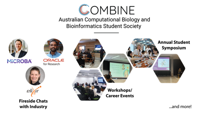
COMBINE is a national student society for students in computational biology, bioinformatics, and related fields. COMBINE is the student subcommittee of The Australian Bioinformatics And Computational Biology Society (ABACBS) as well as the official International Society for Computational Biology (ISCB) Regional Student Group (RSG) for Australia. We aim to bring together students and early-career researchers from the computational and life sciences for networking, collaboration, and professional development. We hold regular workshops, career events, seminars and a yearly symposium, with hundreds of active attendees across Australia and internationally.

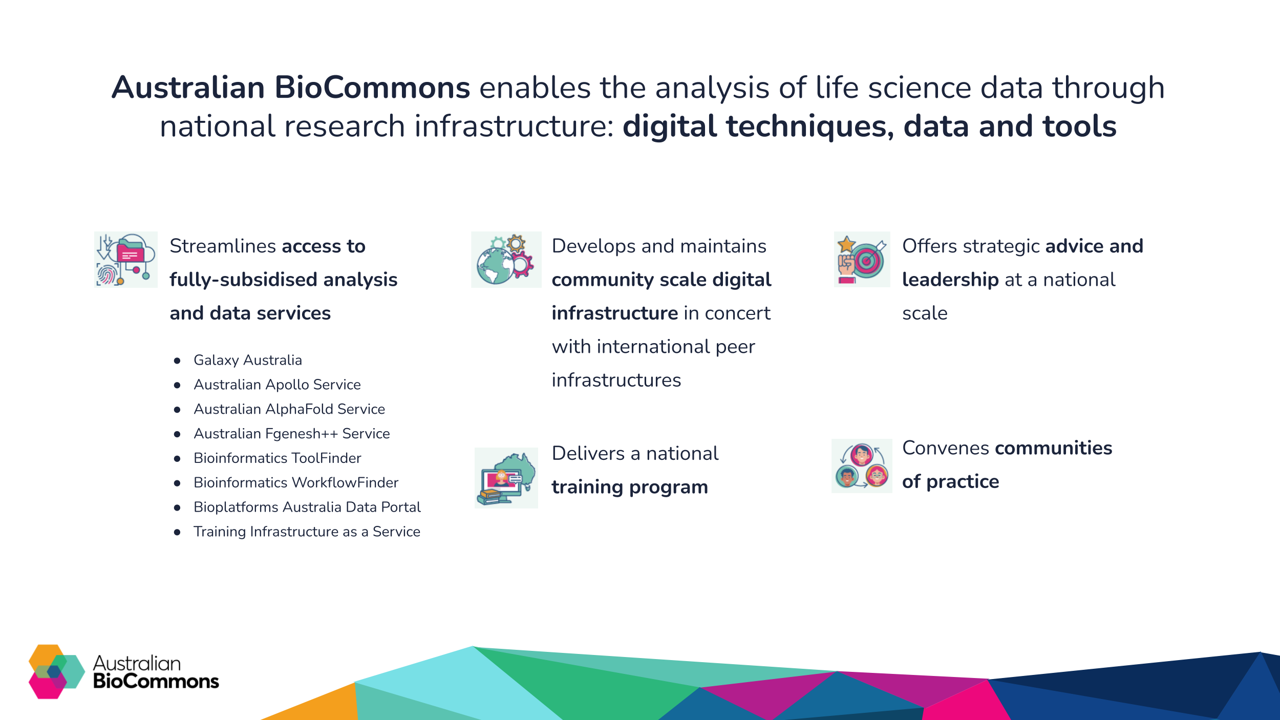
Australian BioCommons is a project that actively supports Australian life scientists by providing national scale research infrastructure. BioCommons is enabled by Australian Government via Bioplatforms Australia funding under the National Collaborative Research Infrastructure Strategy. BioCommons services are fully subsidised for Australian researchers and students to use. BioCommons also delivers bioinformatics training at a national scale through a wide array of webinars, workshops and events that keep participants connected to the latest skills and global developments.

Date and time

12-15 November, 2023.

Location

The 22nd International Conference on Bioinformatics, Translational Research Institute (TRI), Brisbane, Australia.

Instructors and contributors to lesson material

Tyrone Chen , Monash University, Australia
Navya Tyagi , University of Delhi, India
Sonika Tyagi , Royal Melbourne Institute of Technology, Australia

Learning objectives

• Understanding of basic concepts in machine learning

• Describe the unique challenges in biological NLP compared to conventional NLP

• Understand common representations of biological data

• Understand common biological data preprocessing steps

• Investigate biological sequence data for use in machine learning

• Perform a hyperparameter sweep, training and cross-validation

• Identify what the model is focusing on

• Compare trained model performances to each other

Prerequisite knowledge

• [required] Command Line Interface (e.g. bash shell) usage

• [optional] Connecting and working on a remote server (e.g. ssh)

• [optional] Basic knowledge of machine learning

• [optional] Machine learning dashboards (e.g. tensorboard, wandb)

• [optional] Package/environment managers (e.g. conda, mamba)

Intended audience: machine learning practitioners OR computational biologists

Duration

Length: 4.0 hours

Subject	Time	Notes
Introductory lecture	30 min	Lecture
Setup and preprocessing data	45 min	Interactive
Running machine learning	45 min	Interactive
Break	30 min	Break
Cross validation	30 min	Interactive
Comparing and interpreting models	30 min	Interactive
Question and answer	30 min	Interactive

Outline of workshop content

The primary focus of this tutorial is an introduction to machine learning for biological applications. We explore application of NLP in a genomic context by introducing our package genomenlp. In this tutorial, we cover a wide range of topics from introduction to field of GenomeNLP to practical application skills of our anaconda package, divided into various sections:

1. Introduction to machine learning in a biological context

2. Connection to a remote server

3. Installing conda and genomenlp package

4. Setting up a biological dataset

5. Format a dataset as input for genomenlp

6. Preparing a hyperparameter sweep

7. Selecting optimal parameters

8. With the selected hyperparameters, train the full dataset

9. Performing cross-validation

10. Comparing performance of different models

11. Obtain model interpretability scores

For detailed usage of individual functions, please refer to the documentation.

Glossary

• BERT - Bidirectional Encoder Representations from Transformers, a family of deep learning architectures used for NLP.

• DL - Deep Learning

• k-mers - Subunits of a string used as input into conventional NLP algorithms. In this context, k-mers, tokens and words refer to the same thing.

• k-merisation - A process where a biological sequence is segmented into substrings. Commonly performed as a sliding window.

• ML - Machine Learning

• NLP - Natural Language Processing

• OOV - Out-of-vocabulary words

• Sliding window - ABCDEF: [ABC, BCD, CDE, DEF] instead of [ABC, DEF]

• Tokenisation - A process where a string is segmented into substrings

• Tokens - Subunits of a string used as input into conventional NLP algorithms. In this context, k-mers, tokens and words refer to the same thing.

1. Introduction

Introduction to machine learning

View slides here.

What is NLP and genomics

Natural Language Processing (NLP) is a branch of computer science focused around the understanding of and the processing of human language. Such a task is non-trivial, due to the high variation in meaning of words found embedded in different contexts. Nevertheless, NLP is applied with varying degrees of success in various fields, including speech recognition, machine translation and information extraction. A recent well-known example is ChatGPT.

Meanwhile, genomics involves the study of the genome, which contains the entire genetic content of an organism. As the primary blueprint, it is an important source of information and underpins all biological experiments, directly or indirectly.

Why apply NLP in genomics

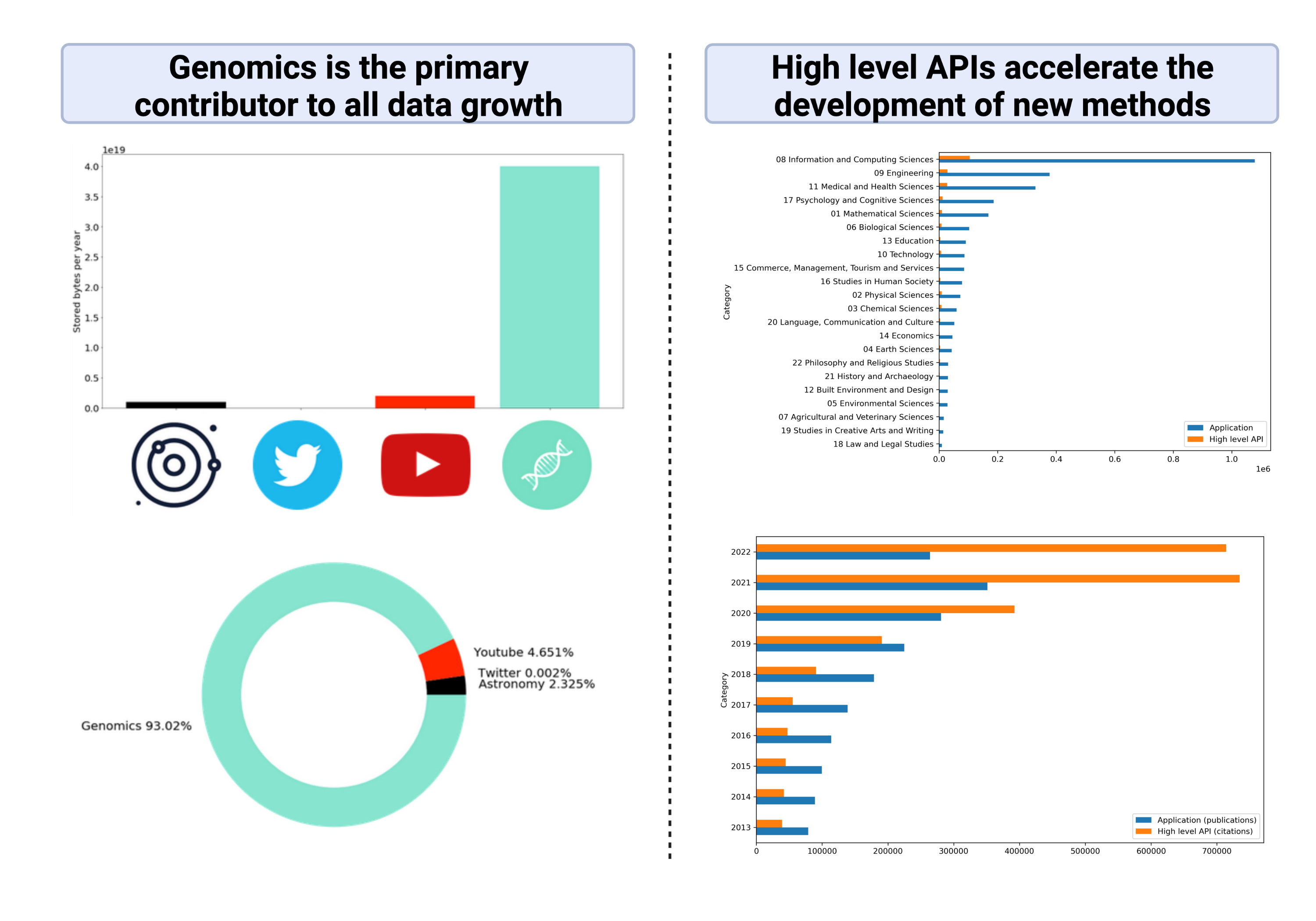
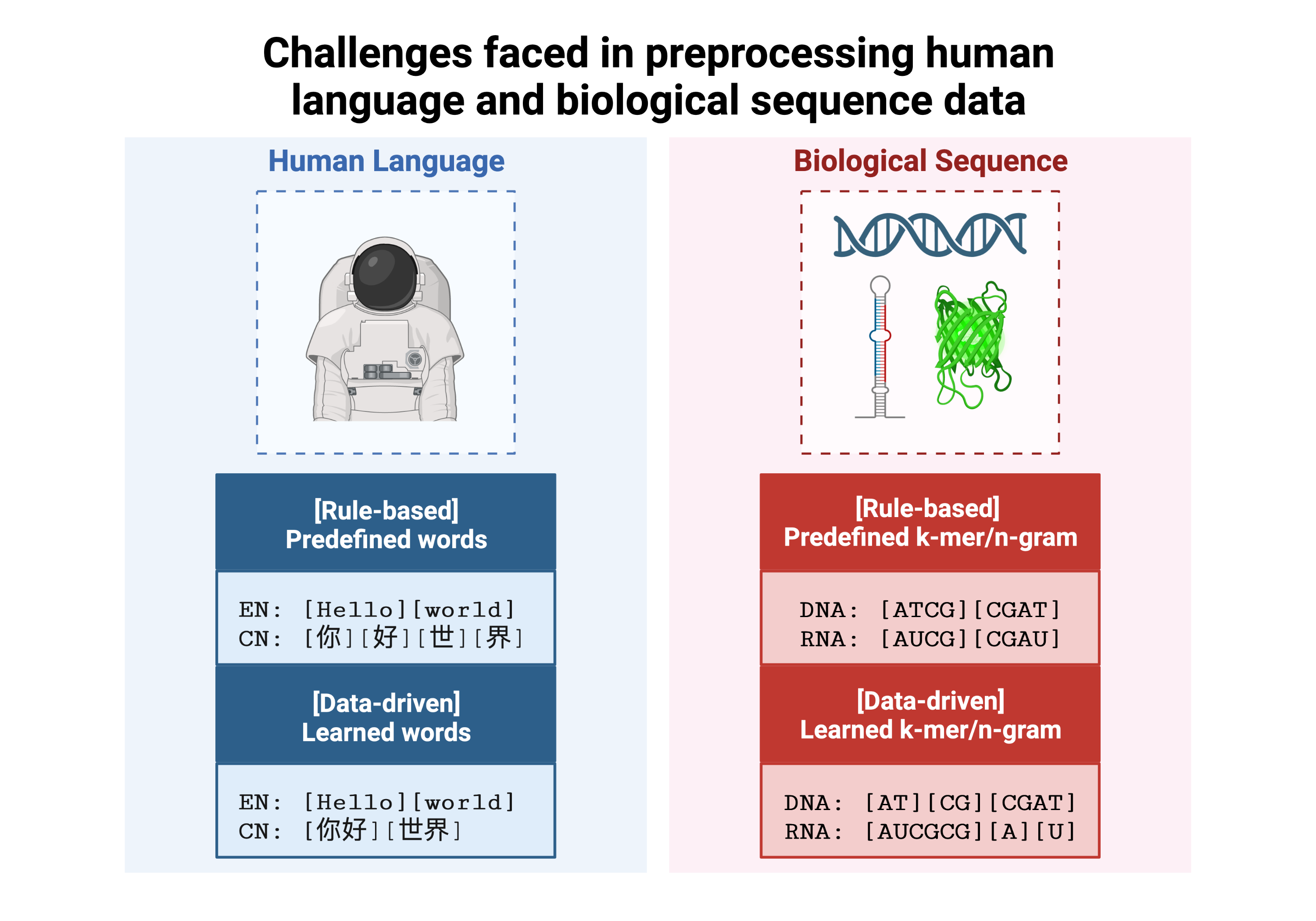
Although NLP has been shown to effectively preprocess and extract “meaning” from human language, until recently, its application in biology was mostly centred around biological literature and electronic health record mining. However, we note the striking similarities between genomic sequence data and human languages that make it well-suited to NLP. (A) DNA can be directly expressed as human language, being composed of text strings such as A, C, T, G, and having its own semantics as well as grammar. (B) Large quantities of biological data are available in the public domain, with a growth rate exponentially exceeding astronomy and social media platforms combined. (C) Recent advances in machine learning which improve the scalability of deep learning (DL) make computational analysis of genomic data feasible.

Note

The same is true for protein sequences, and nucleic acid data such as transcripts. While our pipeline can process any of these, the scope of this tutorial is for genomic data only.

We therefore make a distinction between the field of conventional literature or electronic health record mining and the application of NLP concepts and methods to the genome. We call this field genome NLP. The aim of genome NLP would be to extract relevant information from the large corpora of biological data generated by experiments, such as gene names, point mutations, protein interactions and biological pathways. Applying concepts used in NLP can potentially enhance the analysis and interpretation of genomic data, with implications for research in personalised medicine, drug discovery and disease diagnosis.

Distinction between conventional NLP and genome NLP

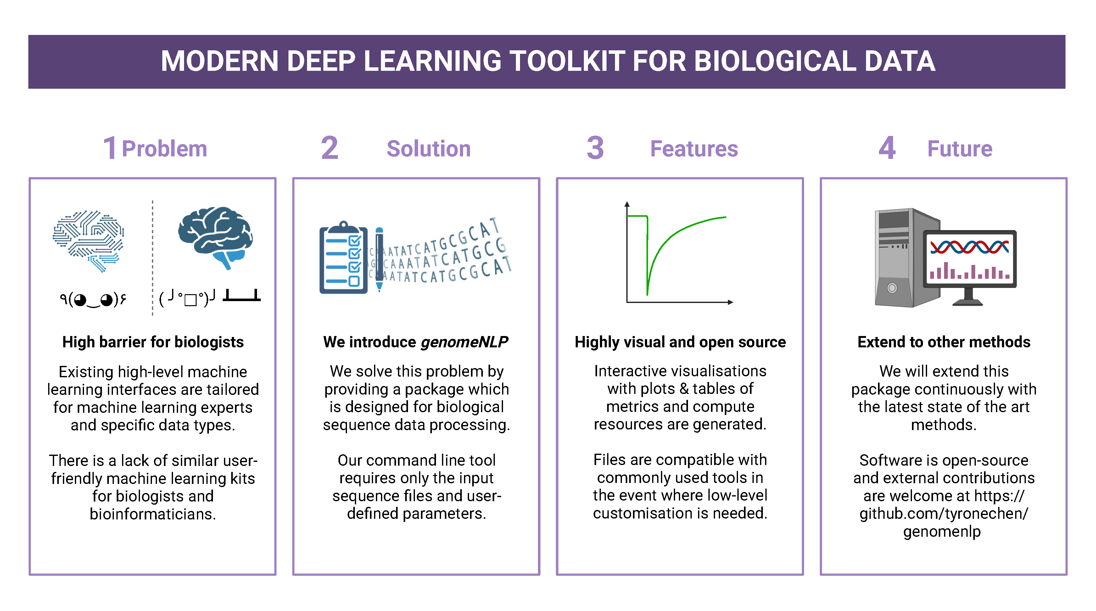
Several key differences need to be accounted for for implementing NLP on the genome. (A) The first challenge is the tokenisation of long biological sequences into smaller subunits. While some natural languages have subunits separated by spaces, enabling easy segmentation, this is not true in biological sequence data, and this also applies to an extent in many languages such as Arabic, Chinese or Sanskrit characters. (B) A second challenge is the diversity and high degree in nuance of biological experiments. As a result, interpretability and interoperability of biological data is highly restricted in scope, even within a single experiment. (C) The third challenge is the difficulty in comparing models, partly due to the second challenge, and partly due to the lack of accessible data in the biomedical field for privacy reasons, and partly because of the limited enforcement of biological data integrity as well as metadata by journals. In addition, the large volume of biological data in a single experiment makes re-training time consuming.

To address the challenges in genome-NLP, we used a new semi-automated workflow. This workflow integrates feature engineering and machine learning techniques and is designed to be adaptable across different species and biological sequences, including nucleic acids and proteins. The workflow includes the introduction of a (1) new tokeniser for biological sequence data which effectively tokenises contiguous genomic sequences while retaining biological context. This minimises manual preprocessing, reduces vocabulary sizes, and (2) handles unknown biological terms, conceptually identical to the out-of-vocabulary (OOV) problem in natural languages. (3) Passing the preprocessed data to a genomicBERT algorithm allows for direct biological sequence input to a state-of-the-art deep learning algorithm. (4) We also enable model comparison by weights, removing the need for computationally expensive re-training or access to raw data. To promote collaboration and adoption, genomicBERT is available as part of the publicly accessible conda package called genomeNLP. Successful case studies have demonstrated the effectiveness of genomeNLP in genome NLP applications.

2. Connect to a remote server

Note

If you are unable to access the command line, you can follow the workshop using jupyter notebooks. Navigate to https://colab.research.google.com, select the GitHub tab, and paste this link https://github.com/tyronechen/genomenlp/blob/main/src/jupyter/case_study_dna.ipynb

To standardise the compute environment for all participants, we will be establishing a network connection with a remote server. Data and a working install of genomenlp is provided. Secure Shell (SSH) is a common method for remote server connection, providing secure access and remote command execution through encrypted connections between the client and server.

Note

Login details will be provided by instructors on the day of the workshop. If you have problems logging in, please contact the instructor.

To use ssh (Secure Shell) for remote server access, please follow these steps:

1. Open a Terminal or Command Prompt on your local machine. SSH is typically available on Unix-like systems (e.g. Linux, macOS) and can also be installed on Windows systems using tools like PuTTY or MobaXterm.

2. Determine the ssh command syntax. Generally the format is: ssh username@hostname or the IP address of the remote server.

3. Enter your password or passphrase when prompted. Once authenticated, you should be connected to the remote server via SSH.

Note

Details for (2) and (3) will be provided on the day of the workshop.

Please login using one user from this list. If you are using ssh, “ssh userID@IPADDRESS” where you replace ID and IPADDRESS from this list. Note that one person can only use one userID and IPADDRESS combination. This is a temporary server provided by Australian BioCommons and will be removed after today.

IF you choose not to use this, you can also follow in google colaboratory or watch the lecture.

3. Installing conda, mamba and genomenlp

Note

This step is already performed for you. Information is provided as a guide for those who are reading this document outside of the tutorial, or if for some reason the installation is not working.

A package/environment manager is a software tool that automates the installation, update, and removal of packages and allows for the creation of isolated environments with specific configurations. This simplifies software setup, reduces compatibility issues, and improves software development workflows. Popular examples include apt and anaconda. We will use conda and mamba in this case study.

Note

The same is true for protein sequences, and nucleic acid data such as transcripts. While our pipeline can process any of these, the scope of this tutorial is for genomic data only.

To install conda using the command line, you can follow these steps:

1. Open your command prompt. Use the curl or wget command to download the installer directly from the command line using its URL.

$ wget 'https://repo.anaconda.com/miniconda/Miniconda3-py39_23.3.1-0-Linux-x86_64.sh'

2. Run the installer script using the following command:

$ bash Miniconda3-py39_23.3.1-0-Linux-x86_64.sh

3. Follow the on-screen prompts to proceed with the installation. (In the prompt asking for the location for conda installation, please specify the directory as foo/bar)

4. Reload your shell as shown below OR exit and return to complete the install.

$ source ~/.bashrc
$ source ~/.bash_profile

5. To install mamba, which is a faster alternative to Conda for package management, run the following command:

$ conda install mamba -n base -c conda-forge

Note

`pip` does not work due to a missing pytorch dependency. `conda` is very slow due to the large dependency tree.

6. As with Step 4, reload your shell as below OR exit and return to complete the install.

$ source ~/.bashrc
$ source ~/.bash_profile

7. To install and activate genomenlp, run the following commands:

$ mamba create -n genomenlp -c tyronechen -c conda-forge genomenlp -y
$ mamba activate genomenlp
# after the above completes
$ sweep -h
# you should see some output

4. Setting up a biological dataset

Understanding of the data and experimental design is a necessary first step to analysis. In our case study, we perform a simple two case classification, where the dataset consists of a corpora of biological sequence data belonging to two categories. Genomic sequence associated with promoters and non-promoter regions are available. In the context of biology, promoters are important modulators of gene expression, and most are relatively short as well as information rich. Motif prediction is an active, on-going area of research in biology, since many of these signals are weak and difficult to detect, as well as varying in frequency and distribution across different species. Therefore, our aim is to classify sequences into promoter and non-promoter sequence categories.

Note

A more detailed description of the data is available here.

Our data is available in the form of fasta files. fasta files are a common format for storing biological sequence data. They typically contain headers that provide information about the sequence, followed by the sequence itself. They can also store other nucleic acid data, as well as protein. The fasta format contains headers with a leading >. Lines without > contain biological sequence data and can be newline separated. In our simple example, the full set of characters are the DNA nucleotides adenine A, thymine T, cytosine C and guanine G. These are the building blocks of the genetic code.

The files can be downloaded here for non promoter sequences and promoter sequences.

# create the directory structure
cd ~
mkdir -p data src results
cd data
curl -L -O "https://raw.githubusercontent.com/tyronechen/genomenlp/main/docs/data/non_promoter.fasta"
curl -L -O "https://raw.githubusercontent.com/tyronechen/genomenlp/main/docs/data/promoter.fasta"
gzip non_promoter.fasta
gzip promoter.fasta

HEADER:   >PCK12019 FORWARD 639002 STRONG
SEQUENCE: TAGATGTCCTTGATTAACACCAAAAT
HEADER:   >ECK12066 REVERSE 3204175 STRONG
SEQUENCE: AAAGAAAATAATTAATTTTACAGCTG

Note

In real world data, other characters are available which refer to multiple possible nucleotides, for example ``W`` indicates either an ``A`` or a ``T``. RNA includes the character ``U``, and proteins include additional letters of the alphabet.

Tokenisation in genomics involves segmenting biological sequences into smaller units, called tokens (or k-mers in biology) for further processing. In the context of genomics, tokens can represent individual nucleotides, k-mers, codons, or other biologically meaningful segments. Just as in conventional NLP, tokenisation is required to facilitate most downstream operations.

Here, we provide gzipped fasta file(s) as input. While conventional biological tokenisation splits a sequence into arbitrary-length segments, empirical tokenisation derives the resulting tokens directly from the corpus, with vocabulary size as the only user-defined parameter. Data is then split into training, testing and/or validation partitions as desired by the user and automatically reformatted for input into the deep learning pipeline.

Note

We provide the conventional k-merisation method as well as an option for users. In our pipeline specifically, the empirical tokenisation and data object creation is split into two steps, while k-merisation combines both in one operation. This is due to the empirical tokenisation process having to “learn” tokens from the data.

# Empirical tokenisation pathway
cd ~/src
tokenise_bio \
  -i ../data/promoter.fasta.gz \
     ../data/non_promoter.fasta.gz \
  -t ../data/tokens.json
# -i INFILE_PATHS path to files with biological seqs split by line
# -t TOKENISER_PATH path to tokeniser.json file to save or load data

This generates a json file with tokens and their respective weights or IDs. You should see some output like this.

[00:00:00] Pre-processing sequences
[00:00:00] Suffix array seeds
[00:00:14] EM training
Sample input sequence: AACCGGTT
Sample tokenised: [156, 2304]
Token: : k-mer map: 156  : : AA
Token: : k-mer map: 2304 : : CCGGTT

5. Format a dataset for input into genomeNLP

In this section, we reformat the data to meet the requirements of our pipeline which takes specifically structured inputs. This intermediate data structure serves as the foundation for downstream analyses and facilitates seamless integration with the pipeline. Our pipeline contains a method that performs this automatically, generating a reformatted dataset with the desired structure.

Note

The data format is identical to that used by the HuggingFace ``datasets`` and ``transformers`` libraries.

# Empirical tokenisation pathway
create_dataset_bio \
  ../data/promoter.fasta.gz \
  ../data/non_promoter.fasta.gz \
  ../data/tokens.json \
  -o ../data/
# -o OUTFILE_DIR write dataset to directory as
#   [ csv \| json \| parquet \| dir/ ] (DEFAULT:"hf_out/")
# default datasets split: train 90%, test 5% and validation set 5%

The output is a reformatted dataset containing the same information. Properties required for a typical machine learning pipeline are added, including labels, customisable data splits and token identifiers.

DATASET AFTER SPLIT:
DatasetDict ({
  train: Dataset ({
  features: ['idx', 'feature', 'labels', 'input_ids', 'token_type_ids', 'attention_mask’],
  num_rows: 12175 })
  test: Dataset ({
  features: ['idx', 'feature', 'labels', 'input_ids', 'token_type_ids', 'attention_mask’],
  num_rows: 677 })
  valid: Dataset ({
  features: ['idx', 'feature', 'labels', 'input_ids', 'token_type_ids', 'attention_mask’],
  num_rows: 676 })
})

Note

The column ``token_type_ids`` is not actually needed in this specific case study, but it is safely ignored in such cases.

SAMPLE TOKEN MAPPING FOR FIRST 5 TOKENS IN SEQ:
TOKEN ID: 858  | TOKEN: TCA
TOKEN ID: 2579 | TOKEN: GCATCAC
TOKEN ID: 111  | TOKEN: TATT
TOKEN ID: 99   | TOKEN: CAGG
TOKEN ID: 777  | TOKEN: AGGCT

6. Preparing a hyperparameter sweep

In machine learning, achieving optimal model performance often requires finding the right combination of hyperparameters (assuming the input data is viable). Hyperparameters vary depending on the specific algorithm and framework being used, but commonly include learning rate, dropout rate, batch size, number of layers and optimiser choice. These parameters heavily influence the learning process and subsequent performance of the model.

For this reason, hyperparameter sweeps are normally carried out to systematically test combinations of hyperparameters, with the end goal of identifying the configuration that produces the best model performance. Usually, sweeps are carried out on a small partition of the data only to maximise efficiency of compute resources, but it is not uncommon to perform sweeps on entire datasets. Various strategies, such as grid search, random search, or bayesian optimisation, can be employed during a hyperparameter sweep to sample parameter values. Additional strategies such as early stopping can also be used.

To streamline the hyperparameter optimization process, we use the wandb (Weights & Biases) platform which has a user-friendly interface and powerful tools for tracking experiments and visualising results.

First, sign up for a wandb account at: https://wandb.ai/site and login by pasting your API key.

wandb login
wandb: Paste an API key from your profile, and hit enter and hit enter or press ctrl+c to quit:

Note

If you are running this on jupyter notebooks, the field to paste the API key is present but invisible (click the space just after the most recent output).

Now, we use the sweep tool to perform hyperparameter sweep. Search strategy, parameters and search space are passed in as a json file. An example is below. If no sweep configuration is provided, default configuration will apply.

Default hyperparameter sweep settings if none are provided. You can copy this file and edit it for your own use if needed.

{
    "name": "random",
    "method": "random",
    "metric": {
        "name": "eval/f1",
        "goal": "maximize"
        },
    "parameters": {
        "epochs": {
            "values": [1, 2, 3, 4, 5]
            },
        "dropout": {
          "values": [0.15, 0.2, 0.25, 0.3, 0.4]
        },
        "batch_size": {
            "values": [8, 16, 32, 64]
            },
        "learning_rate": {
            "distribution": "log_uniform_values",
            "min": 1e-5,
            "max": 1e-1
        },
        "weight_decay": {
            "values": [0.0, 0.1, 0.2, 0.3, 0.4, 0.5]
        },
        "decay": {
            "values": [1e-5, 1e-6, 1e-7]
        },
        "momentum": {
            "values": [0.8, 0.9, 0.95]
        }
    },
    "early_terminate": {
        "type": "hyperband",
        "s": 2,
        "eta": 3,
        "max_iter": 27
    }
}

sweep \
  ../data/train.parquet \
  parquet \
  ../data/tokens.json \
  -t ../data/test.parquet \
  -v ../data/valid.parquet \
  -w ../data/hyperparams.json \   # optional
  -e entity_name \       # <- edit as needed
  -p project_name \      # <- edit as needed
  -l labels \
  -n 3
# -t TEST, path to [ csv \| csv.gz \| json \| parquet ] file
# -v VALID, path to [ csv \| csv.gz \| json \| parquet ] file
# -w HYPERPARAMETER_SWEEP, run a hyperparameter sweep with config from file
# -e ENTITY_NAME, wandb team name (if available).
# -p PROJECT_NAME, wandb project name (if available)
# -l LABEL_NAMES, provide column with label names (DEFAULT: "").
# -n SWEEP_COUNT, run n hyperparameter sweeps

*****Running training*****
Num examples = 12175
Num epochs= 1
Instantaneous batch size per device = 64
Total train batch size per device = 64
Gradient Accumulation steps= 1
Total optimization steps= 191

The output is written to the specified directory, in this case sweep_out and will contain the output of a standard pytorch saved model, including some wandb specific output.

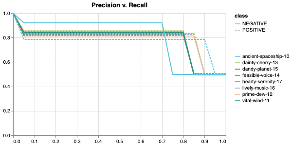
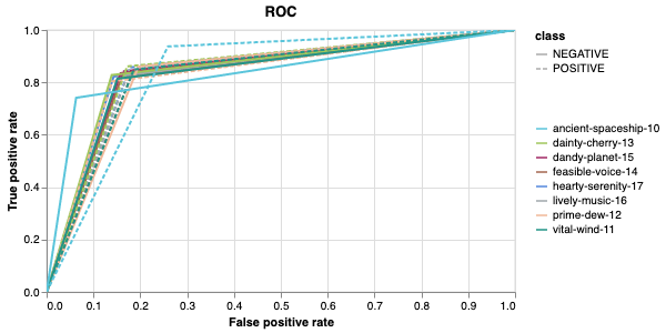
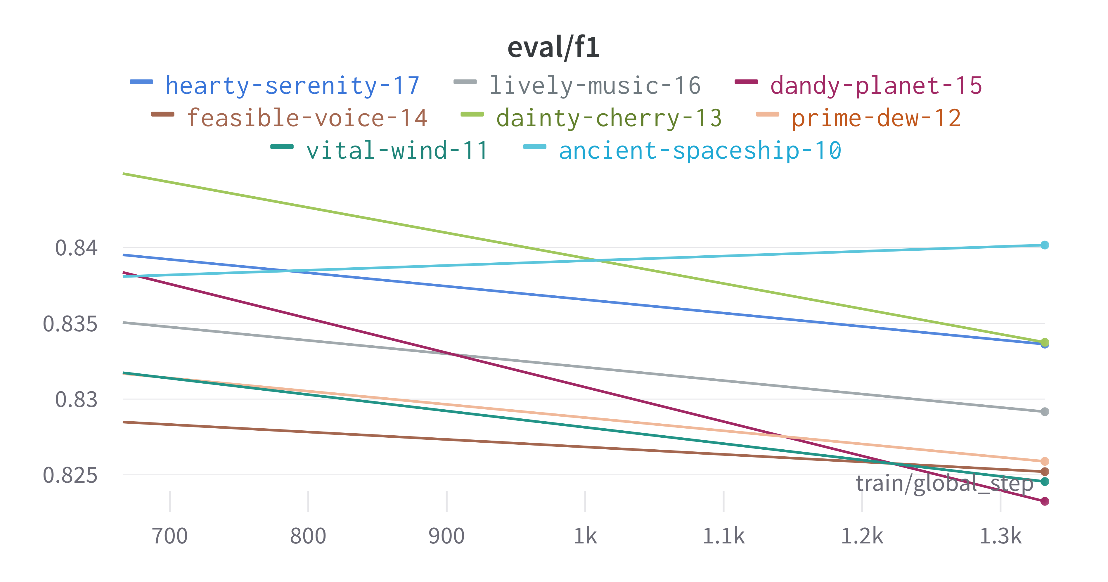
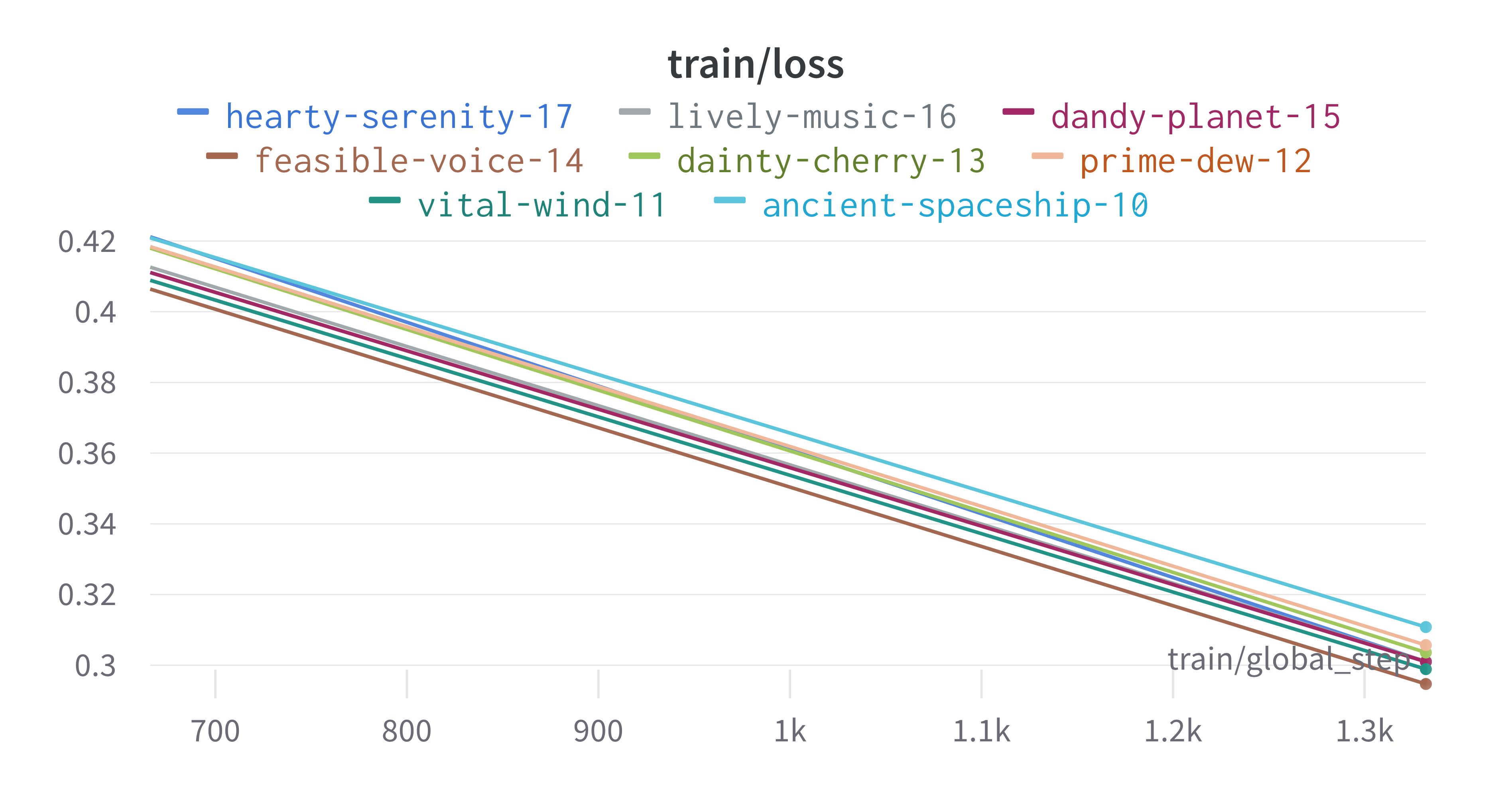
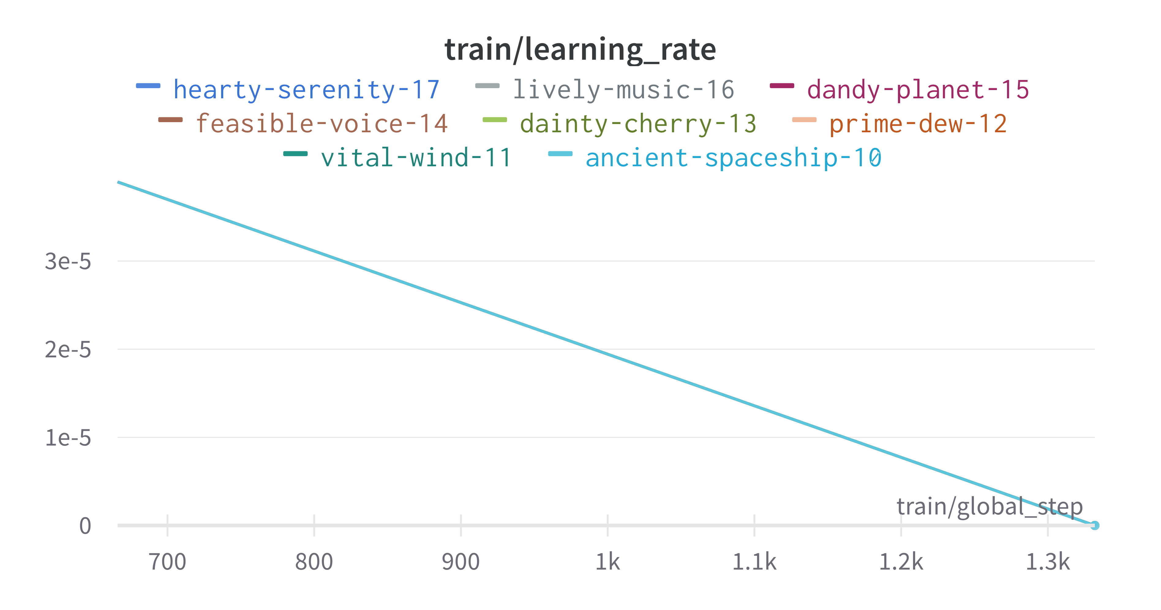
The sweeps gets synced to the wandb dashboard along with various interactive custom charts and tables which we provide as part of our pipeline. A small subset of plots are provided for reference. Interactive versions of these and more plots are available on wandb.

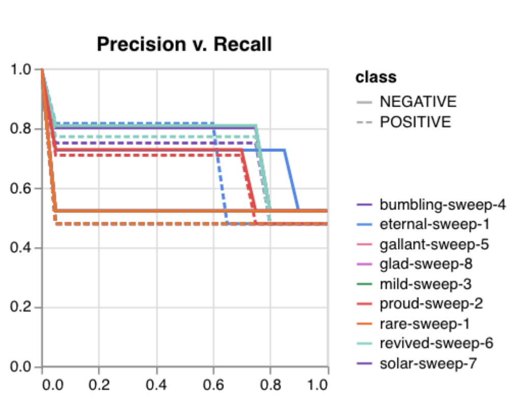
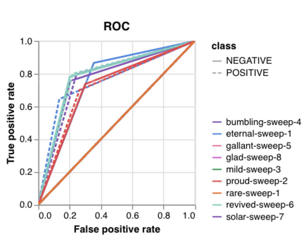
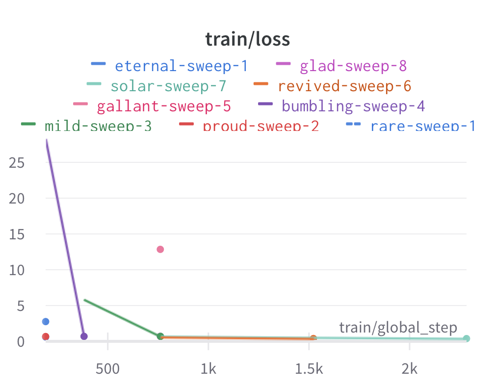
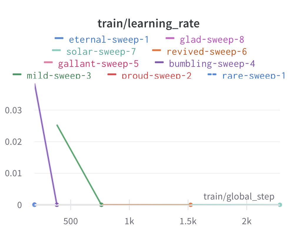
Here is an example of a full wandb generated report:

You may inspect your own generated reports after they complete.

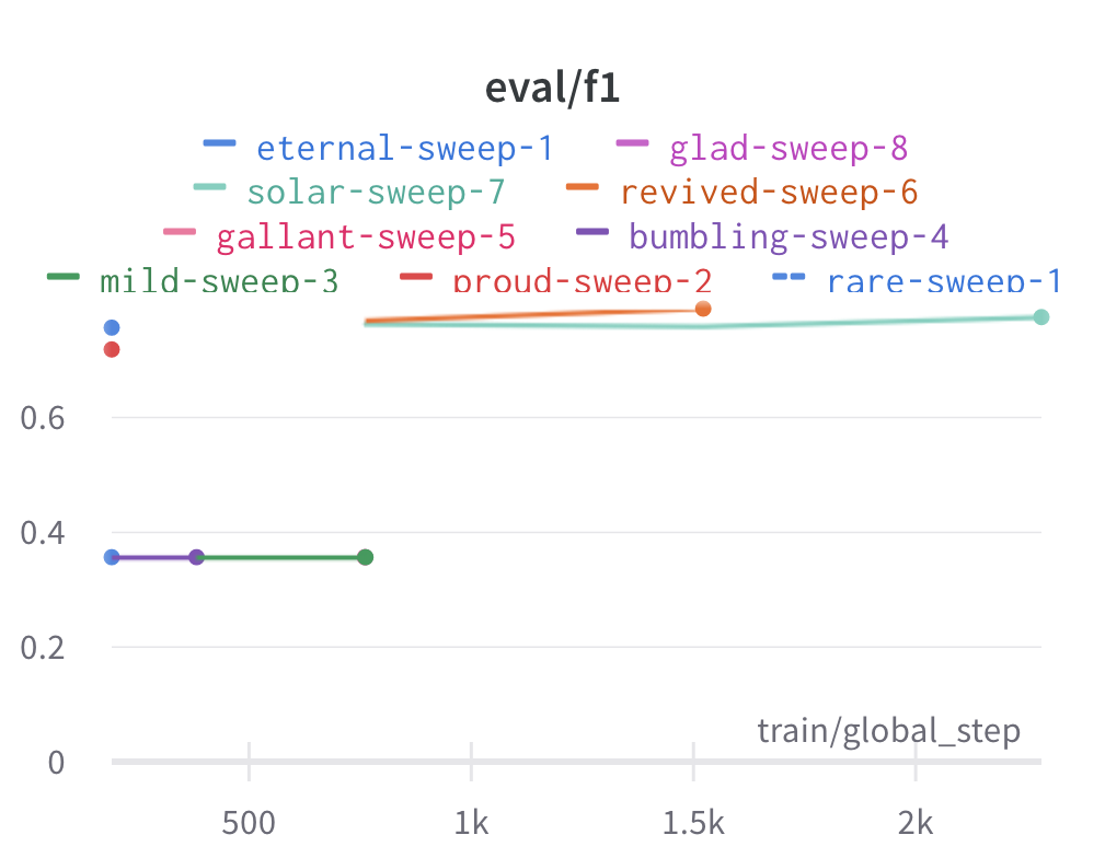
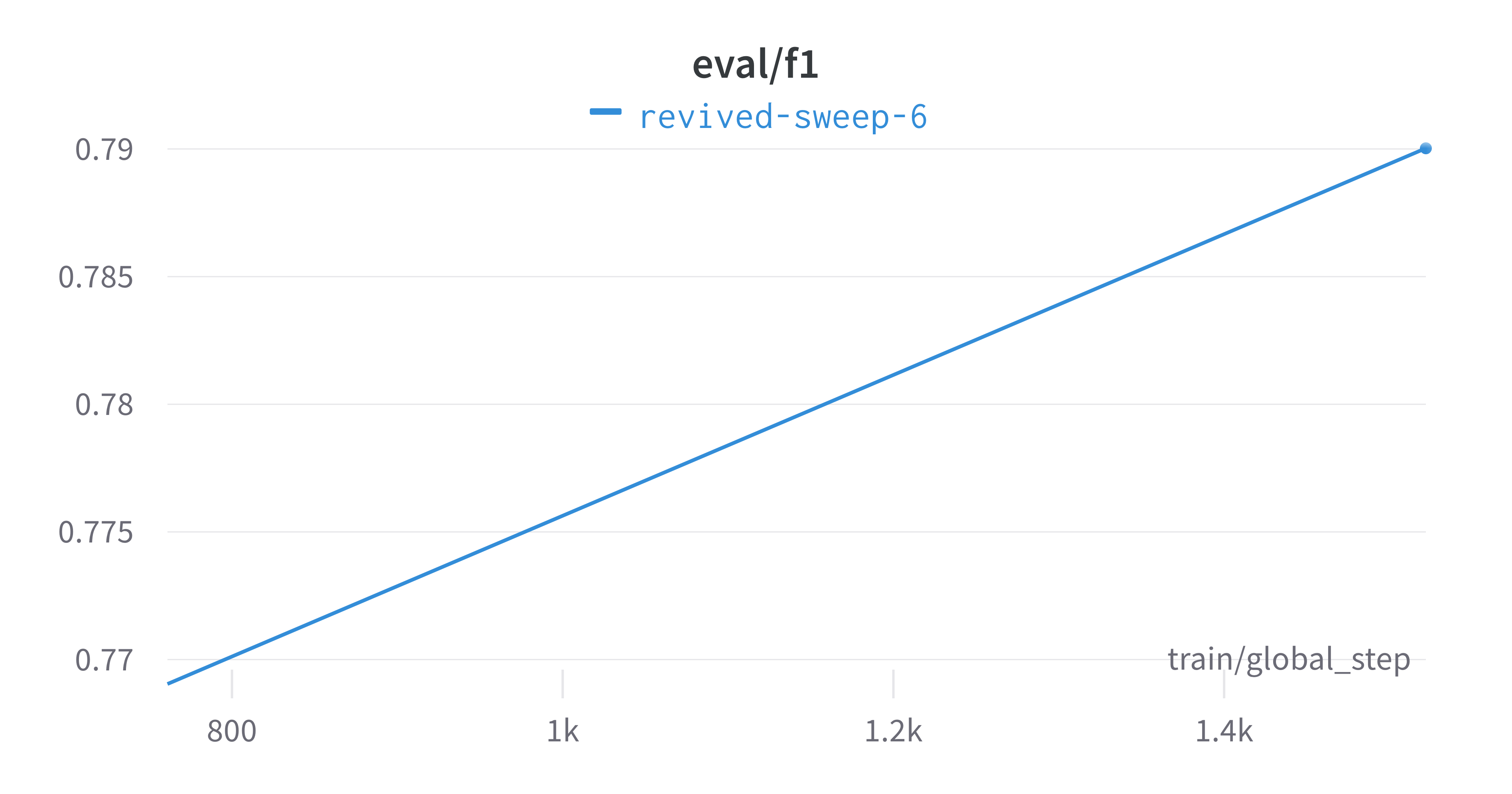
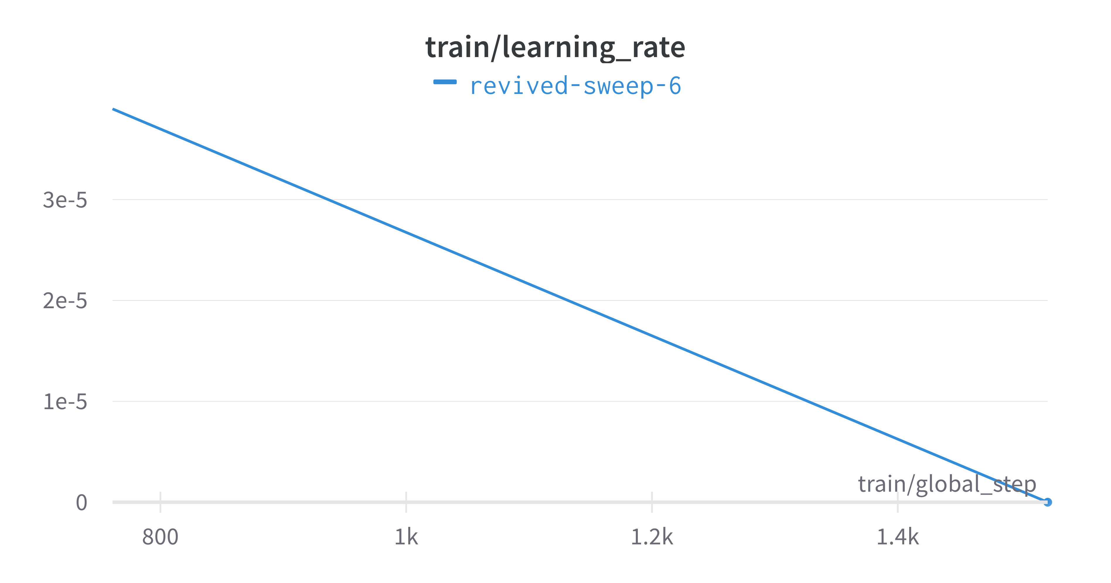
7. Selecting optimal hyperparameters for training

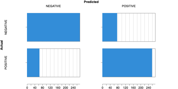
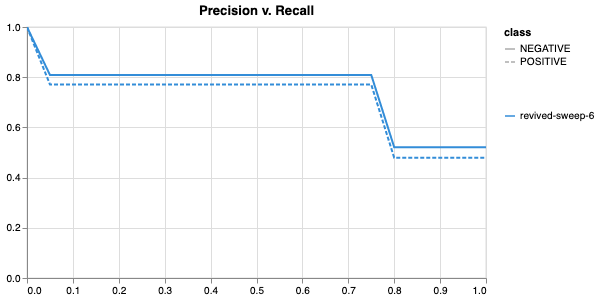
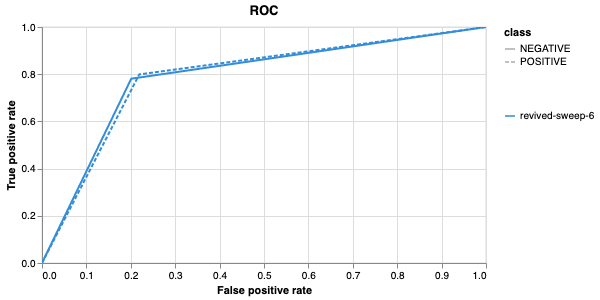
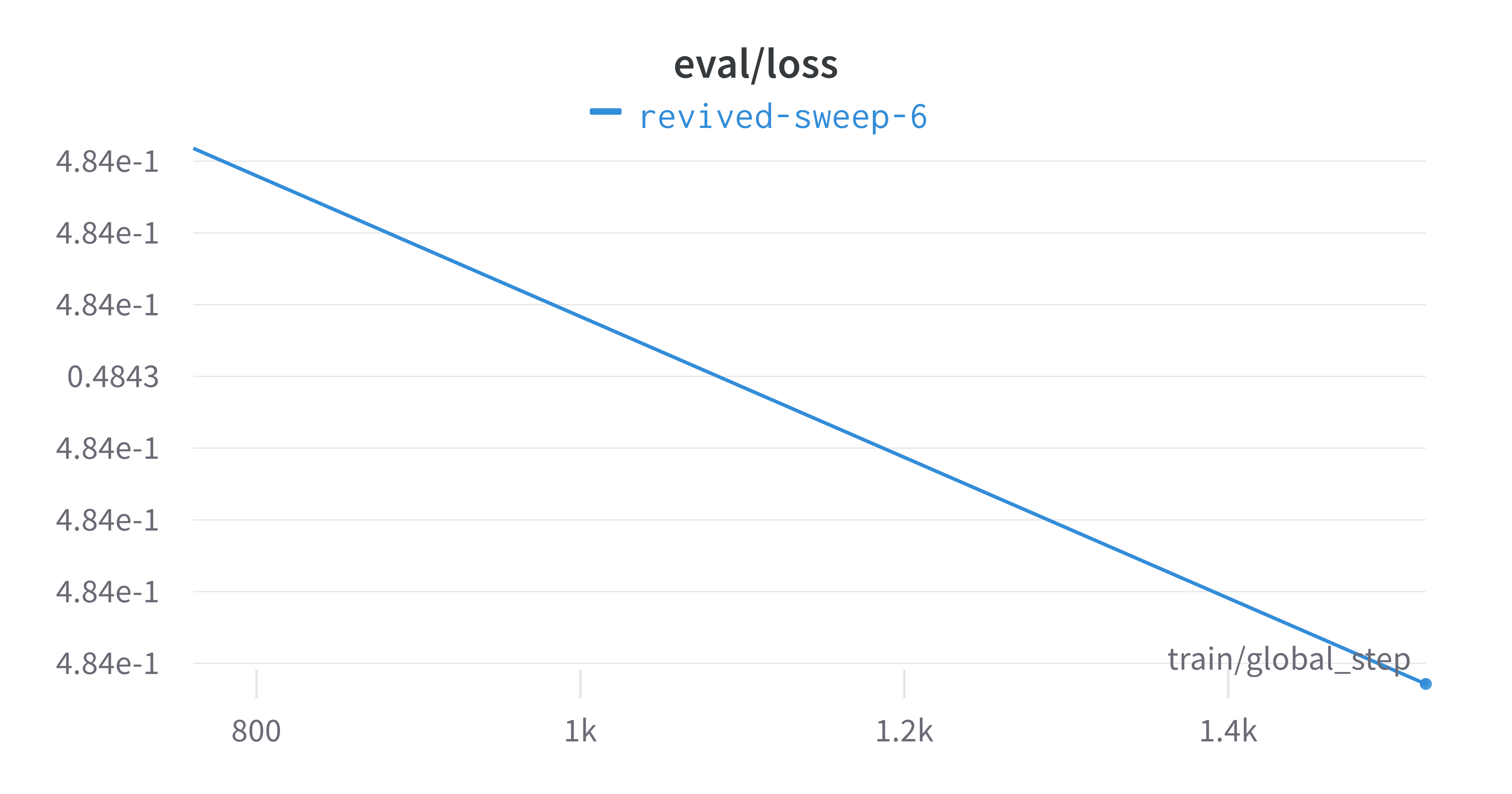
Having completed a sweep, we next identified the best set of parameters for model training. We do this by examining training metrics. These serve as quantitative measures of a model’s performance during training. These metrics provide insights into the model’s accuracy and generalisation capabilities. We explore commonly used training metrics, including accuracy, loss, precision, recall, and f1 score to inform us of a model’s performance

A key event we want to avoid is overfitting. Overfitting occurs when a learning model performs exceptionally well on the training data but fails to generalise to unseen data, making it unfit for use outside of the specific scope of the experiment. This can be detected by observing performance metrics, if the accuracy decreases and later increases an overfit event has occurred. In real world applications, this can lead to adverse events that directly impact us, considering that such models are used in applications such as drug prediction or self-driving cars. Here, we use the f1 score calculated on the testing set as the main metric of interest. We showed that we obtain a best f1 score of 0.79.

Best run revived-sweep-6 with eval/f1=0.7900291349379833
BEST MODEL AND CONFIG FILES SAVED TO: *./sweep_out/model_files*
HYPERPARAMETER SWEEP END

Here is an example of a full wandb generated report for the “best” run.

You may inspect your own generated reports after they complete.

8. With the selected hyperparameters, train the full dataset

In a conventional workflow, the sweep is performed on a small subset of training data. The resulting parameters are then recorded and used in the actual training step on the full dataset. Here, we perform the sweep on the entire dataset, and hence remove the need for further training. If you perform this on your own data and want to use a small subset, you can do so and then pass the recorded hyperparameters with the same input data to the train function of the pipeline. We include an example of this below for completeness, but you can skip this for our specific case study. Note that the input is almost identical to sweep.

train \
  ../data/train.parquet \
  parquet \
  ../data/tokens.json \
  -t ../data/test.parquet \
  -v ../data/valid.parquet \
  --output_dir ../results/train_out \
  -f ../data/hyperparams.json \  # <- you can pass in hyperparameters
  -c entity_name/project_name/run_id \  # <- wandb overrides hyperparameters
  -e entity_name \   # <- edit as needed
  -p project_name    # <- edit as needed
# -t TEST, path to [ csv \| csv.gz \| json \| parquet ] file
# -v VALID, path to [ csv \| csv.gz \| json \| parquet ] file
# -w HYPERPARAMETER_SWEEP, run a hyperparameter sweep with config from file
# -e ENTITY_NAME, wandb team name (if available).
# -p PROJECT_NAME, wandb project name (if available)
# -l LABEL_NAMES, provide column with label names (DEFAULT: "").

Note

Remove the ``-e entity_name`` line if you do not have a group setup in wandb

The contents of hyperparams.json, the file with the best hyperparameters identified by the sweep.

{
  "output_dir": "./sweep_out/random",
  "overwrite_output_dir": false,
  "do_train": false,
  "do_eval": true,
  "do_predict": false,
  "evaluation_strategy": "epoch",
  "prediction_loss_only": false,
  "per_device_train_batch_size": 16,
  "per_device_eval_batch_size": 16,
  "per_gpu_train_batch_size": null,
  "per_gpu_eval_batch_size": null,
  "gradient_accumulation_steps": 1,
  "eval_accumulation_steps": null,
  "eval_delay": 0,
  "learning_rate": 7.796477400405317e-05,
  "weight_decay": 0.5,
  "adam_beta1": 0.9,
  "adam_beta2": 0.999,
  "adam_epsilon": 1e-08,
  "max_grad_norm": 1.0,
  "num_train_epochs": 2,
  "max_steps": -1,
  "lr_scheduler_type": "linear",
  "warmup_ratio": 0.0,
  "warmup_steps": 0,
  "log_level": "passive",
  "log_level_replica": "passive",
  "log_on_each_node": true,
  "logging_dir": "./sweep_out/random/runs/out",
  "logging_strategy": "epoch",
  "logging_first_step": false,
  "logging_steps": 500,
  "logging_nan_inf_filter": true,
  "save_strategy": "epoch",
  "save_steps": 500,
  "save_total_limit": null,
  "save_on_each_node": false,
  "no_cuda": false,
  "use_mps_device": false,
  "seed": 42,
  "data_seed": null,
  "jit_mode_eval": false,
  "use_ipex": false,
  "bf16": false,
  "fp16": false,
  "fp16_opt_level": "O1",
  "half_precision_backend": "auto",
  "bf16_full_eval": false,
  "fp16_full_eval": false,
  "tf32": null,
  "local_rank": -1,
  "xpu_backend": null,
  "tpu_num_cores": null,
  "tpu_metrics_debug": false,
  "debug": [],
  "dataloader_drop_last": false,
  "eval_steps": null,
  "dataloader_num_workers": 0,
  "past_index": -1,
  "run_name": "./sweep_out/random",
  "disable_tqdm": false,
  "remove_unused_columns": false,
  "label_names": null,
  "load_best_model_at_end": true,
  "metric_for_best_model": "loss",
  "greater_is_better": false,
  "ignore_data_skip": false,
  "sharded_ddp": [],
  "fsdp": [],
  "fsdp_min_num_params": 0,
  "fsdp_transformer_layer_cls_to_wrap": null,
  "deepspeed": null,
  "label_smoothing_factor": 0.0,
  "optim": "adamw_hf",
  "adafactor": false,
  "group_by_length": false,
  "length_column_name": "length",
  "report_to": [
    "wandb"
  ],
  "ddp_find_unused_parameters": null,
  "ddp_bucket_cap_mb": null,
  "dataloader_pin_memory": true,
  "skip_memory_metrics": true,
  "use_legacy_prediction_loop": false,
  "push_to_hub": false,
  "resume_from_checkpoint": null,
  "hub_model_id": null,
  "hub_strategy": "every_save",
  "hub_token": "<HUB_TOKEN>",
  "hub_private_repo": false,
  "gradient_checkpointing": false,
  "include_inputs_for_metrics": false,
  "fp16_backend": "auto",
  "push_to_hub_model_id": null,
  "push_to_hub_organization": null,
  "push_to_hub_token": "<PUSH_TO_HUB_TOKEN>",
  "mp_parameters": "",
  "auto_find_batch_size": false,
  "full_determinism": false,
  "torchdynamo": null,
  "ray_scope": "last",
  "ddp_timeout": 1800
}

The output is written to the specified directory, in this case train_out and will contain the output of a standard pytorch saved model, including some wandb specific output.

The trained model gets synced to the wandb dashboard along with various interactive custom charts and tables which we provide as part of our pipeline. A small subset of plots are provided for reference. Interactive versions of these and more plots are available on wandb.

Here is an example of a full wandb generated report:

You may inspect your own generated reports after they complete.

9. Perform cross-validation

Having identified the best set of parameters and trained the model, we next want to conduct a comprehensive review of data stability, and we do this by evaluating model performance across different data slices. This assessment is known as cross-validation. We make use of k-fold cross-validation in which data is divided into k subsets and the model is trained and tested on these individual subsets.

cross_validate \
  ../data/train.parquet parquet \
  -t ../data/test.parquet \
  -v ../data/valid.parquet \
  -e entity_name \              # <- edit as needed
  -p project_name \             # <- edit as needed
  --config_from_run p9do3gzl \  # id OR directory of best performing run
  --output_dir ../results/cv \
  -m ../results/sweep_out \     # <- overridden by --config_from_run
  -l labels \
  -k 8
# --config_from_run WANDB_RUN_ID, *best run id*
# –-output_dir OUTPUT_DIR
# -l label_names
# -k KFOLDS, run n number of kfolds

cross_validate \
  ../data/train.parquet parquet \
  -t ../data/test.parquet \
  -v ../data/valid.parquet \
  -e tyagilab \
  -p foobar \
  -c tyagilab/foobar/kixu82co \
  -o ../results/cv \
  -m ../results/sweep_out \
  -l labels \
  -k 8

Note

If both ``model_path`` and ``config_from_run`` are specified, ``config_from_run`` overrides

Note

Remove the ``-e entity_name`` line if you do not have a group setup in wandb

*****Running training*****
Num examples = 10653
Num epochs= 2
Instantaneous batch size per device = 16
Total train batch size (w, parallel, distributed & accumulation)= 16
Gradient Accumulation steps= 1
Total optimization steps= 1332
Automatic Weights & Biases logging enabled

The cross-validation runs are uploaded to the wandb dashboard along with various interactive custom charts and tables which we provide as part of our pipeline. These are conceptually identical to those generated by sweep or train. A small subset of plots are provided for reference. Interactive versions of these and more plots are available on wandb.

Here is an example of a full wandb generated report:

You may inspect your own generated reports after they complete.

10. Compare different models

The aim of this step is to compare performance of different deep learning models efficiently while avoiding computationally expensive re-training and data download in conventional model comparison. In the case of patient data, they are often inaccessible for privacy reasons, and in other cases they are not uploaded by the authors of the experiment.

For the purposes of this simple case study, we compare multiple sweeps of the same dataset as a demonstration. In a real life application, existing biological models can be compared against the user-generated one.

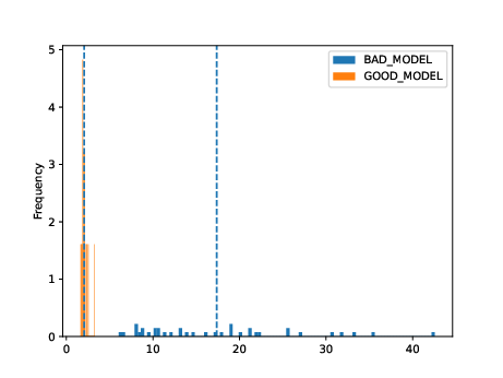
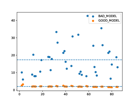
fit_powerlaw \
  ../results/sweep_out/model_files \
  -o ../results/fit
# -m MODEL_PATH, path to trained model directory
# -o OUTPUT_DIR, path to output metrics directory

This tool outputs a variety of plots in the specified directory.

ls ../results/fit
# alpha_hist.pdf  alpha_plot.pdf  model_files/

Very broadly, the overlaid bar plots allow the user to compare the performance of different models on the same scale. A narrow band around 2-5 with few outliers is in general cases an indicator of good model performance. This is a general guideline and will differ depending on context! For a detailed explanation of these plots, please refer to the original publication.

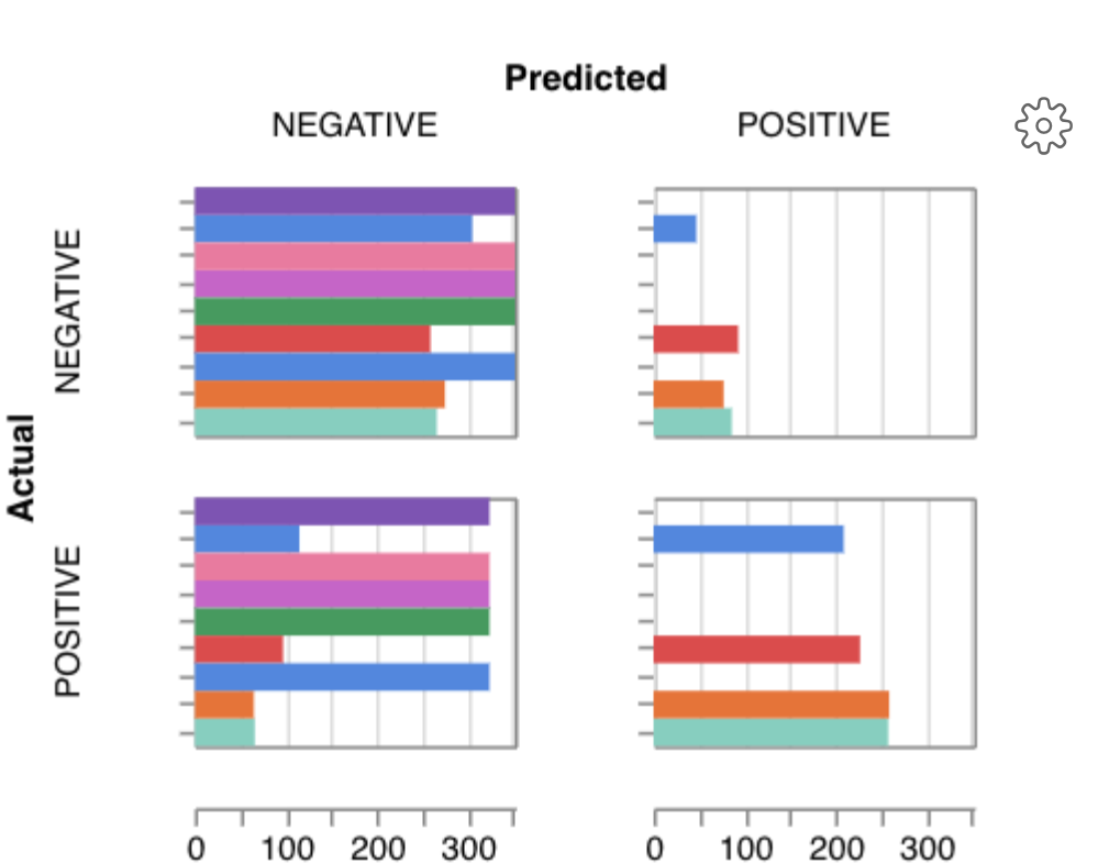
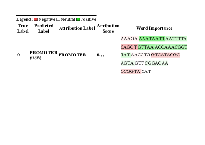
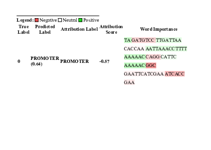
11. Obtain model interpretability scores

Model interpretability is often used for debugging purposes, by allowing the user to “see” (to an extent) what a model is focusing on. In this case, the tokens which contribute to a certain classification are highlighted. The green colour indicates a classification towards the target category, while the red colour indicates a classification away from the target category. Colour intensity indicates the classification score.

In some scenarios, we can exploit this property by identifying regulatory regions or motifs in DNA sequences, or discovering amino acid residues in protein structure critical to its function, leading to a deeper understanding of the underlying biological system.

gzip -cd ../data/promoter.fasta.gz | \
  head -n10 > ../data/subset.fasta
interpret \
  ../results/sweep_out/model_files \
  ../data/subset.fasta \
  -l PROMOTER NON-PROMOTER \
  -o ../results/model_interpret
# -t TOKENISER_PATH, path to tokeniser.json file to load data
# -o OUTPUT_DIR, specify path for output

ECK120010480 CSGDP1 REVERSE 1103344 SIGMA38.html
ECK120010489 OSMCP2 FORWARD 1556606 SIGMA38.html
ECK120010491 TOPAP1 FORWARD 1330980 SIGMA32 STRONG.html
ECK120010496 YJAZP  FORWARD 4189753 SIGMA32 STRONG.html
ECK120010498 YADVP2 REVERSE 156224  SIGMA38.html

12. Interactive question and answer session

Citation

Cite our manuscript here:

@article{chen2023genomicbert,
    title={genomicBERT and data-free deep-learning model evaluation},
    author={Chen, Tyrone and Tyagi, Navya and Chauhan, Sarthak and Peleg, Anton Y and Tyagi, Sonika},
    journal={bioRxiv},
    month={jun},
    pages={2023--05},
    year={2023},
    publisher={Cold Spring Harbor Laboratory},
    doi={10.1101/2023.05.31.542682},
    url={https://doi.org/10.1101/2023.05.31.542682}
}

Cite our software here:

@software{tyrone_chen_2023_8135591,
  author       = {Tyrone Chen and
                  Navya Tyagi and
                  Sarthak Chauhan and
                  Anton Y. Peleg and
                  Sonika Tyagi},
  title        = {{genomicBERT and data-free deep-learning model
                  evaluation}},
  month        = jul,
  year         = 2023,
  publisher    = {Zenodo},
  version      = {latest},
  doi          = {10.5281/zenodo.8135590},
  url          = {https://doi.org/10.5281/zenodo.8135590}
}